Carbon Dioxide: Projected emissions and concentrations
Storylines and emissions
The greenhouse gas forcing used by the AR4 models are derived from SRES emissions scenarios. The SRES report discusses emissions projections produced by a range of Integrated Assessment Models for a range of socio-economic storylines. Four ‘marker scenarios’ are recommended as the basis of climate model projections, together with two further ‘illustrative scenarios’:
| Storyline | Integrated Assessment Model | Status |
| A1 (A1B) | AIM | Marker |
| A2 | ASF | Marker |
| B1 | IMAGE | Marker |
| B2 | MESSAGE | Marker |
| A1T | MESSAGE | Illustrative |
| A1FI | MINICAM (A1G) | Illustrative |
The projected emissions for the marker scenarios and other scenarios discussed in the SRES report are available here.
Note that the A1FI set of scenarios was formed as a union of the A1G and A1C scenario groups: in some documents the A1FI MINICAM illustrative scenario is referred to as the A1G MINICAM scenario.
Recent increase and projected changes in CO2 concentrations
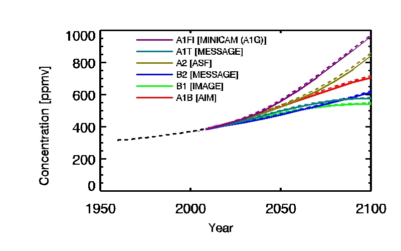
The modern increase in atmospheric CO2 concentration is shown in the Manua Loa time series in figue 1 below. The annual means are plotted, and can be downloaded (here). More data and information on CO2 monitoring is available from the NOAA Earth System Research Laboratory Global Monitoring Division, including monthly data from Mauna Loa.
For each of the illustrative and marker emissions scenarios, CO2 concentration projections calculated by two different carbon cycle models were reported in IPCC WG1 (2001) and used as the bases for climate model projections there and in the Fourth Assessment Report. Thes are also shown in Figure 1. The carbon cycle models, ISAM and BERN, are described in Box 3.7 of IPCC (2001). The projected concentrations are given in Annex II of the IPCC Third Assessment WG I report (the `reference’ projections were used). The data can be obtained as plain text files here: ISAM, BERN.
|
|
Figure 1: Atmospheric CO2 concentrations as observed at Mauna Loa from 1958 to 2008 (black dashed line) and projected under the 6 SRES marker and illustrative scenarios. Two carbon cycle models (see Box 3.7 in IPCC, 2001) are used for each scenario: BERN (solid lines) and ISAM (dashed). |
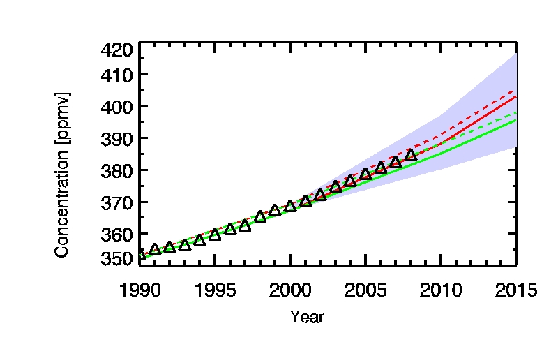
As shown in figure 2, atmospheric CO2 concentrations since 1990 have risen in line with projections from the SRES report, lying close to the highest of illustrative/marker scenarios predicted with the BERN model, and towards the lower limit of the ISAM illustrative/marker scenario projections. The ESRL “annual average marine surface air CO2 concentrations” shown in figure 2 is of shorter duration (starting in 1980), but gives an accurate estimate of the global mean CO2 concentration. The concentrations at Mauna Loa are generally 1 to 2 ppmv lower that the ESRL values. In the time period shown in figure 2 the difference between the carbon cycle models is comparable to the difference between the two extremes of the illustrative/marker scenarios, but later in the century (figure 1) the difference between scenarios dominates. Uncertainties in CO2 concentrations due to the range of possible climate - carbon cycle feedbacks in the BERN and ISAM models are larger than the differences between these two models.
|
|
Figure 2: Observed and projected atmospheric CO2 concentrations since 1990. Triangles show annual average marine surface air CO2 concentrations for the period 1990 to 2008 downloaded from the NOAA ESRL web site (www.esrl.noaa.gov) in September 2009. The red and green lines shows annual average CO2 concentrations for the SRES A1B (red) and B2 (green) marker emissions scenarios projected using the reference version of the Bern carbon cycle model (solid) and the ISAM model (dashed). These two scenarios give the upper and lower limits of the 6 illustrative/marker scenarios in the period plotted. The blue shading shows the range from low to high climate - carbon cycle feedbacks. All SRES projections are taken from Annex B of the 2001 IPCC Working Group I Report. |
Carbon cycle models and GCMs
The carbon cycle model used to generate the forcings used by various AR4 General Circulation Models are listed in the table below:
| Carbon Cycle Model | General Circulation Model |
| ISAM | MRI:CGCM2_3_2; NASA:GISS-AOM, GISS-EH, GISS-ER GFDL:CM2 GFDL:CM2_1 |
| BERN-CC |
BCC:CM1;
BCCR:BCM2;
CNRM:CM3; INM:CM3; IPSL:CM4; LASG:FGOALS-G1_0; NCAR:CCSM3; NIES:MIROC3_2-HI, MIROC3_2-MED; UKMO:HADCM3, HADGEM1 |
Changes in CO2 in the distant past
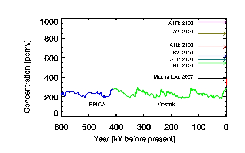
The observed and projected changes in CO2 concentrations can be put into context by comparing them with measurements of past variations. The levels of carbon dioxide in the atmosphere in the distant past can be determined from bubbles of air trapped in ice. Data from the Antarctic sites Vostok and Epica ice cores (see Fig. 6.3 of the IPCC AR4, the physical science basis are plotted together in figure 3. Also shown are the AD2007 annual mean concentration measured at Mauna Loa and the the projected concentrations for AD2100 under 6 SRES marker and illustrative scenarios. The 50 year period of Mauna Loa observations and the century covered by the projections span less than the thickness of a line on this graph.
|
|
Figure 3: CO2 concentrations derived from EPICA and Vostok ice cores. The red bar at the side indicates the evolution of the Mauna Loa measurements. On this time scale, the 50 years of measurements span less than the thickness of the line, so it appears vertical. |